BLAKE2 RTL implementation
Introduction #
In this project we have implemented a feature reduced version of the BLAKE2 cryptographic hash function into
synthesizable RTL using Verilog.
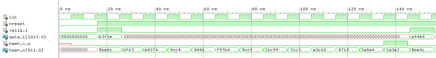
BLAKE2b hash simulation wave view: it takes 12 cycles to produce a result for one block.Blake2 RTL implementation
BLAKE2
#
BLAKE2 is specified in the RFC7693.
The algorithm receives plaintext data, breaks it down into blocks of 32 or 64 bytes
and produces a hash of 16 or 32 bytes for each block.
In practice BLAKE2 is used in different applications from password hashing to proof of work
for cryptocurrencies.
There are 2 main flavors of BLAKE2:
| block size (bytes) | hash size (bytes) | |
|---|---|---|
BLAKE2b | 64 | 32 |
BLAKE2s | 32 | 16 |
Our code is written in a parametric fashion, to support both the b and s flavor.
This hash function works on individual blocks of data or on data streams.
Function overview #
The
BLAKE2
takes plaintext data, breaks it down into blocks of 32 or 64 bytes,
and passes each of these blocks through the
compression function.
The main loop in this function includes the permutation function and the mixing function, this
loop will be called 10 or 12 times.
The number of rounds is dependant of the flavor of BLAKE2 :
| BLAKE2b | BLAKE2s | |
|---|---|---|
| rounds | 12 | 10 |
Permutation function
#
Within the compression function loop, at the start of each round, we calculate a new 16 entry wide selection array s
based on a predefined pattern shown below :
| Round | 0 | 1 | 2 | 3 | 4 | 5 | 6 | 7 | 8 | 9 | 10 | 11 | 12 | 13 | 14 | 15 |
|---|---|---|---|---|---|---|---|---|---|---|---|---|---|---|---|---|
| SIGMA[0] | 0 | 1 | 2 | 3 | 4 | 5 | 6 | 7 | 8 | 9 | 10 | 11 | 12 | 13 | 14 | 15 |
| SIGMA[1] | 14 | 10 | 4 | 8 | 9 | 15 | 13 | 6 | 1 | 12 | 0 | 2 | 11 | 7 | 5 | 3 |
| SIGMA[2] | 11 | 8 | 12 | 0 | 5 | 2 | 15 | 13 | 10 | 14 | 3 | 6 | 7 | 1 | 9 | 4 |
| SIGMA[3] | 7 | 9 | 3 | 1 | 13 | 12 | 11 | 14 | 2 | 6 | 5 | 10 | 4 | 0 | 15 | 8 |
| SIGMA[4] | 9 | 0 | 5 | 7 | 2 | 4 | 10 | 15 | 14 | 1 | 11 | 12 | 6 | 8 | 3 | 13 |
| SIGMA[5] | 2 | 12 | 6 | 10 | 0 | 11 | 8 | 3 | 4 | 13 | 7 | 5 | 15 | 14 | 1 | 9 |
| SIGMA[6] | 12 | 5 | 1 | 15 | 14 | 13 | 4 | 10 | 0 | 7 | 6 | 3 | 9 | 2 | 8 | 11 |
| SIGMA[7] | 13 | 11 | 7 | 14 | 12 | 1 | 3 | 9 | 5 | 0 | 15 | 4 | 8 | 6 | 2 | 10 |
| SIGMA[8] | 6 | 15 | 14 | 9 | 11 | 3 | 0 | 8 | 12 | 2 | 13 | 7 | 1 | 4 | 10 | 5 |
| SIGMA[9] | 10 | 2 | 8 | 4 | 7 | 6 | 1 | 5 | 15 | 11 | 9 | 14 | 3 | 12 | 13 | 0 |
This array s is then used to select the indexes used to access data from our
message block vector m.
In the C language, this operation can be written simply as m[sigma[round][x]], with round the
round we are currently at and x the initial array index.
In hardware, this function is admittedly the most costly component of this entire algorithm as it requires a lot of muxing logic :
One 64 bit wide, 10 deep mux to select, depending on which round we are at, the correct
sselect values. Link to code16 64 bit wide, 16 deep muxes used to assign the new values of array
m, and using values ofsfor the select. Link to code
Mixing function
#
This function is also part of the compression function loop.
It is referred to in the official
specification as G. It takes in 6 bytes and produces 4 new bytes.
FUNCTION G(v[0..15], a, b, c, d, x, y)
    |
    |   v[a] := (v[a] + v[b] + x) mod 2**w
    |   v[d] := (v[d] ^ v[a]) >>> R1
    |   v[c] := (v[c] + v[d])     mod 2**w
    |   v[b] := (v[b] ^ v[c]) >>> R2
    |   v[a] := (v[a] + v[b] + y) mod 2**w
    |   v[d] := (v[d] ^ v[a]) >>> R3
    |   v[c] := (v[c] + v[d])     mod 2**w
    |   v[b] := (v[b] ^ v[c]) >>> R4
    |
    |   RETURN v[0..15]
    |
    END FUNCTION.
Internally it is composed of simple operations :
- 3 way unsigned integer
add - 32 or 64 byte
modulo circular right shiftxor
The G function is called in the compression loop, with the following arguments:
v := G(v, 0, 4,  8, 12, m[s[ 0]], m[s[ 1]])
v := G(v, 1, 5,  9, 13, m[s[ 2]], m[s[ 3]])
v := G(v, 2, 6, 10, 14, m[s[ 4]], m[s[ 5]])
v := G(v, 3, 7, 11, 15, m[s[ 6]], m[s[ 7]])

v := G(v, 0, 5, 10, 15, m[s[ 8]], m[s[ 9]])
v := G(v, 1, 6, 11, 12, m[s[10]], m[s[11]])
v := G(v, 2, 7,  8, 13, m[s[12]], m[s[13]])
v := G(v, 3, 4,  9, 14, m[s[14]], m[s[15]])
In practice we have already obtained the values of x and y from having calculated the values
for m[s[x]] as part of the permutation function.
The values of a, b, c and d are constants.
Values for R1, R2, R3, and R4 depend on the flavor of BLAKE2 we are implementing.
| BLAKE2b | BLAKE2s | |
|---|---|---|
| R1 | 31 | 16 |
| R2 | 24 | 12 |
| R3 | 16 | 8 |
| R4 | 63 | 7 |
As such, this function easily maps onto hardware with minimal cost. Link to code
Testing #
To test our implementation, we are comparing the output of our simulated implementation with the test vector produced by a golden model.
In this case our golden model was the C
implementation of BLAKE2 found in the appendix of the RFC7693 specification.
For more instructions on running the test bench see the README .