I have a confession to make: floating point scares me.
Half a decade ago I decided that I was going to implement some floating point arithmetic. Back then it seemed approachable enough, after all, floating points are ubiquitous. How hard can it really be ? My experience until that point had been: given enough time and effort is spent bashing my brain against a problem, I can generally figure things out.
This is how I faced the most complete technical defeat of my existence. Through this utter annihilation emerged my present fear of floating point.
After half a decade I decided it was time for a rematch, time to face my dragons!
But this time, I would not simply aim for a surface level understanding, this time I would aim to deeply grasp the floating point representation.
When setting out on this crusade, I believed that there were only 3 types of people who truly understood floating point :
- The people writing the spec
- The math PhDs working on the floating point representation
- The people building the floating point hardware
Welcome to round 2!
Chapter 1: Descent into madness#
Looking back on it, one of the main reasons behind my past defeat was that I mistook my ability to use floating points for a marker of understanding. And that this freed me from the need to invest the time in studying floating point, as if I was going to pick it up along the way.
So it’s now time to put the computer aside, and spend 10 days in the company of paper. ( you remember, the white stuff )
How floating point works#
I am assuming that readers already have some surface level knowledge of what floating point is, so I will spare you the basic intro.
Let me just set a few definitions, in the context of this discussion normal floating point numbers will be defined as:
$$ (-1)^{S} × 2^{E−b} × (1 + T \cdot 2^{1−p}) $$With the values of \(S\), \(E\) and \(T\) being the values stored in the floating point fields:
- \(S\) sign bit
- \(E\) biased exponent
- \(T\) trailing significant field
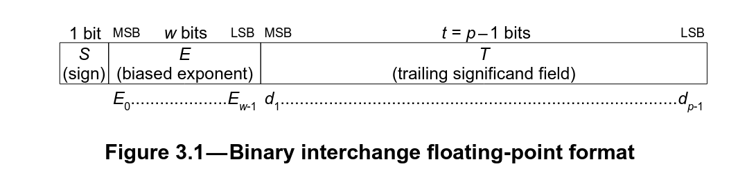
The size of these fields, as well as the values of \(b\) (exponent bias) and \(p\) (precision) depend on the floating point format.
Eg, for the IEEE 754 single precision (float32_t) we have:
- \(b = 127\)
- \(p = 24\)
Resulting in:
$$ (-1)^{S} \times 2^{E−127} \times (1 + T \cdot 2^{-23}) $$In this discussion we will be calling :
- sign, the \(S\) sign bit
- exponent, the value stored in the biased exponent field \(E\)
- significant/mantissa, the value stored in the \(T\) field
The term mantissa isn’t pedantically correct since this isn’t a logarithmic representation it should really be called a significant. But my fellow programmers in the audience will appreciate that since the sign has already used the \(s\) name for our single letter naming of our structure elements we have no choice but to yield and call this \(m\) for mantissa. I will be using the term mantissa and significant interchangeably in this article.
What you never wanted to know#
We are not actually interested in floating point in the abstract, but rather what we commonly refer to as “float” in our programs.
In the world of all the possible floating point types, these are the vanillas, except in this world, everyone also wants vanilla all the time!
This float format is canonized by the IEEE in the IEEE 754 specification. Inside this holy grail is where the expected behavior is outlined in excruciating detail making it possible for users to expect the same behavior for the same floating point operations on different platforms. A cornerstone of making float portable.
Also, this is where hell starts!
+0/-0#
Let us commence our descent slowly.
As the most astute readers might have already noticed looking (kudos) at the representation format, we have a real sign bit. This implies that we actually have 2 representations for zero: \(+0.0\) and \(-0.0\).
Now where things get fun is that we have rules around which zero to use. For example, let us consider how we would determine the equality between two floating point numbers, say X == Y ?
To do this comparison we would generally re-use the adder and do X - Y then check all the result’s bits are 0, problem is \(-0.0\) is written with an 1 in its sign bit.
So we have rules around when the result should use \(+0.0\) or \(-0.0\), and the subtracting of two equal floating point numbers is such an example of this rule :
NaN#
NaN for Not A Number.
For all of you that thought we were talking about numbers, this is the point at which you start understanding the difference between a number and a representation format.
So let’s start with the fun bit, there are actually different types of NaN’s:
quietNaNs (qNaNs) that you would typically encounter from your bad math.signalingNaNs (sNaNs) the ones bad math doesn’t produce and also the ones that scream at you by signaling an invalid operation exception whenever they appear as operands. Most people won’t encounter these.
So, what do I mean by “qNaNs are used to indicate when the result of an arithmetic operation cannot be represented”?
Here are a few examples for clarification :
- \(\sqrt{-1.0}\) results in an
qNaNas \(\sqrt{-1.0} = i\), and \(i\) is an imaginary number that cannot be represented without the use of complex notation. - \(\frac{0.0}{0.0}\) would also result in a
qNaNbecause: what are you doing ? - \(+\infty - \infty\) would also result in a
qNaNbecause \(\pm\infty\) are actually limits, not numbers. And subtracting a limit from another limit \(+\infty - \infty\) just doesn’t make sense.
Want to know another fun fact about qNaNs ?
They are contagious.
Arithmetic operations with a qNaN as an operand will result in a qNaN.
Think about it: what result should you give for an operation whose result can’t be represented ?
In memory NaNs are represented with all the exponent bits set to \(1\) and with at least one of the significant bits set. You can then differentiate different NaNs based on which significant bit(s) are set, the encoding of which is left to the discretion of the implementer.
Infinitys#
So we have already started introducing these with the NaNs, but the floating point representation has room for two infinity notations: one for \(+\infty\) and its mirror \(-\infty\). These are not numbers, infinity is not a number it’s a limit!
In compliance with IEEE certain specific infinities can be used in arithmetic operations, be used as inputs for boolean operations and be produced as the result of a calculation.
In memory, infinities have their exponent bits set to all \(1\)s, and to differentiate them from NaNs their significant bits are all \(0\)s.
Denormal#
Let’s put infinities and NaNs on the side for a minute and get back to talking just about numbers.
In the introduction I defined a normal floating point number as:
A more common way of writing this is:
Where \(m\) is a number represented by a string of the form \(d_0 . d_1 d_2 ... d_{p-1}\), and is \(p\) long.(with \(p\) the precision, or number of bits in the significant + 1 ).
For example \(1.5\) would be written as :
and \(3\) as \(2 × 1.5\) :
In our normal floating point representation, the \(1\) in \((1 + T · 2^{1−p})\) is our \(d_0\) and is always set to \(d_0 = 1\).
Now, the funny thing is our significant actually only has \(p-1\) bits, and \(d_0\) is actually an inferred bit, we call it the hidden bit.
Seems simple enough ? Could something finally be simple about floating point ?!
Don’t worry: floating point isn’t going to let you down like this, because we have another category of numbers!
They have an implicit hidden bit set to \(d_0 = 0\) and are called subnormal numbers (or denormal numbers). Yay 🥳
These are used to encode the smallest representable floating point numbers, and were the most controversial part of the IEEE 574 spec during its elaboration.
They are also a giant pain in the ass to implement, so much so that a lot of the early FPU’s would trap on subnormal numbers and handle them in software … very slowly …
So why are we putting up with them apart from not wanting to waste some bits ?
The culprit: gradual underflow.
Gradual underflow#
The idea behind gradual underflow is to slow the loss of precision instead of it being abrupt after the smallest representable normal number: \(2^{-(b+1)-p+1}\). This helps with numerical stability.
To illustrate what I mean, let’s imagine we didn’t have subnormals, \(x\) and \(y\) where floating points numbers such that \(x \neq y\). If \(x - y\) fell in the range between \(0.0\) and the smallest representable floating point number then it would underflow to \(0.0\) since there is no representable number in that range.
Eg, using float16 without subnormals:
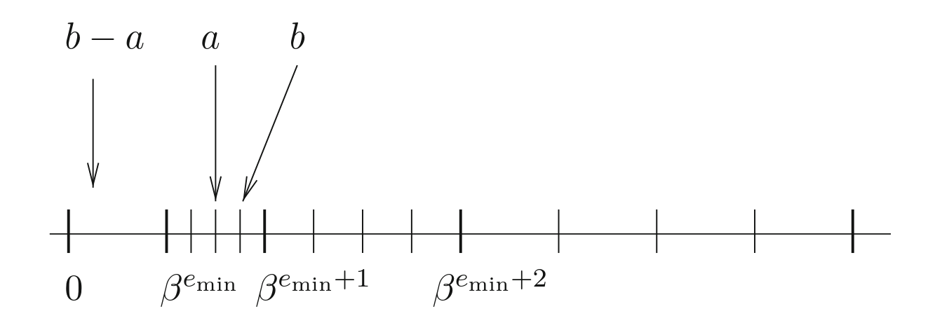
Now when we add subnormals we are effectively filling this gap.
Eg,using float16 with subnormals:
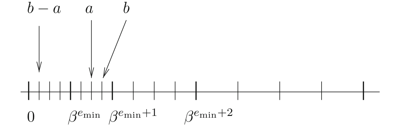
Now with subnormals in our system we inherit the following interesting property: for any floating point number \(x\) and \(y\) such that \(x \neq y\), \(x - y\) is necessarily nonzero.
Bonus: we have now acquired extra armour against a division by zero:
if ( x != y ) z = 1.0 / ( x - y );
Rounding modes#
The range of what can and cannot be represented is type specific, more bits equates to a larger space of representable values, conversely smaller types mean less possible values.
Let us consider the IEEE 16 bit half float float16_t , it has 5 exponent bits and 10 significant bits, and guess what : it can’t represent 15359!
So what would happen when we try to set it to 15359 ?
float16_t e = 15359.0;
cout << e << endl;
The answer is 42.
More seriously, it depends: what rounding mode are we using ?
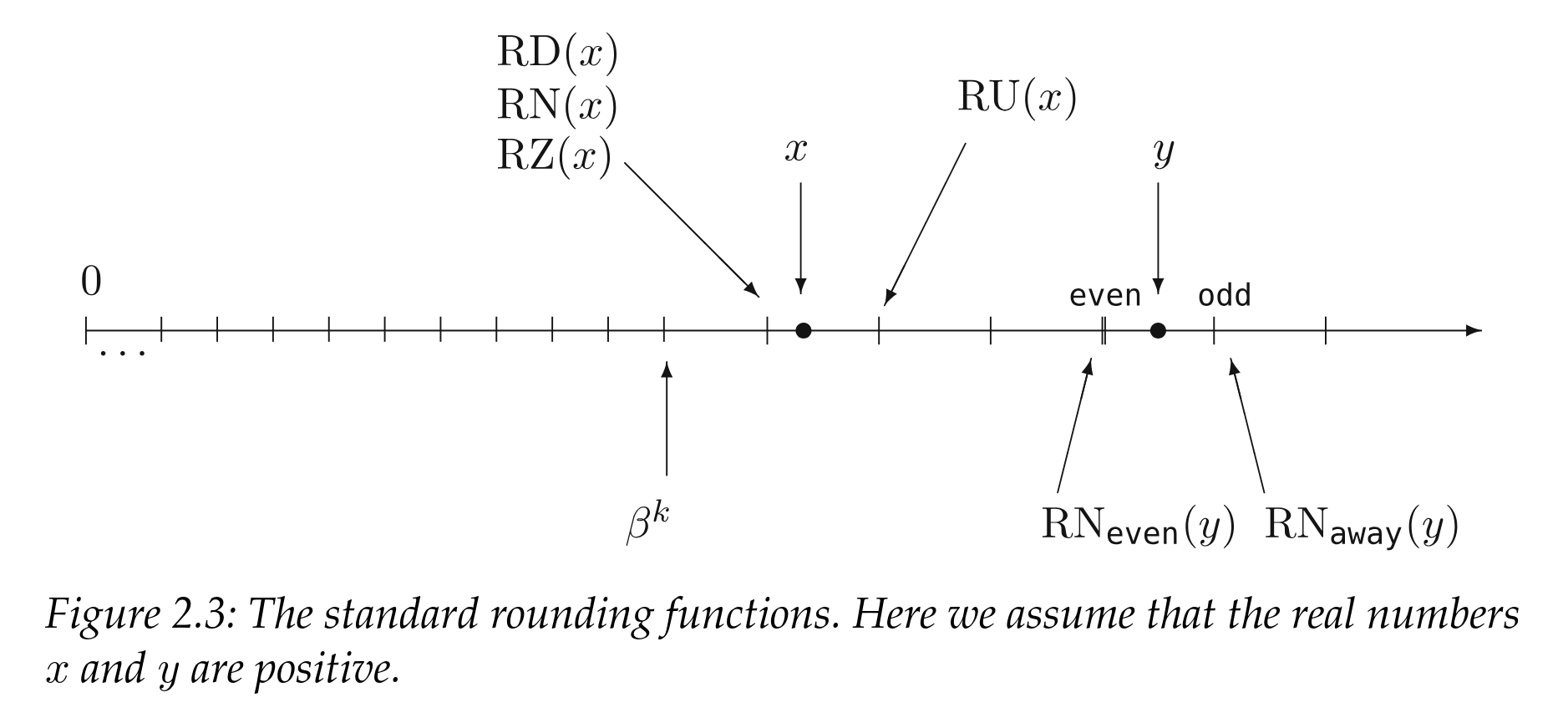
The IEEE spec defines 5 rounding modes that compliant hardware should support:
RDround downwards towards \(-\infty\): the result is the largest representable floating point less than or equal to the exact resultsRUround towards \(+\infty\): the result is the smallest representable floating point greater or equal to the exact resultsRZround towards \(0.0\) in all casesRN_even/RN_awayround to nearest: the result is the nearest possible value, with a tie breaking rule if the number is exactly halfway between the two:even(round ties to even) chooses the number where the least significant bit of the significant ( mantissa) is 0.away(round ties to away) chooses the next consecutive floating point number.
Let us get back to our example, 15359 isn’t a representable number with a float16_t, and the closest two numbers are 15352 and 15360.
So depending on which rounding mode we are using we will get :
| rounding mode | result |
|---|---|
| RD | 15352 |
| RZ | 15352 |
| RU | 15360 |
| RN (even) | 15360 |
RN_even is the default IEEE rounding mode behavior on modern systems and is what is specified by the C++ FE_TONEAREST rounding mode.
Rounding modes boundary behavior#
Recall how, when I was describing the behavior of the rounding modes I didn’t systematically use the term “number” for the rounding result ? This is because some rounding modes cause the result to round into \(\pm\infty\).
For example on float16_t using RU rounding :
float16_t x, y, z;
x = 65504;
y = 1;
fesetround(FE_UPWARD);
z = x + y;
cout << x << " + " << y << " = " << z << endl;
Would result in :
65504 + 1 = inf Similarly :
float16_t x, y, z;
x = -65504;
y = 1;
fesetround(FE_DOWNWARD);
z = x - y;
cout << x << " - " << y << " = " << z << endl;
Would round down to \(-\infty\) :
-65504 - 1 = -inf Conjunctly these definitions imply that operations using the RU will never reach \(-\infty\) and operations using RD will never reach \(+\infty\).
float16_t x, y, zsub, zadd;
x = 65504;
y = 1;
fesetround(FE_UPWARD);
zsub = -x - y;
cout << -x << " - " << y << " = " << zsub << endl;
fesetround(FE_DOWNWARD);
zadd = x + y;
cout << x << " + " << y << " = " << zadd << endl;
Result :
-65504 - 1 = -65504
65504 + 1 = 65504
Now where this get’s fun is with RZ , since it behaves like a RD for positive numbers and a RU on negative numbers, this means operations using this rounding mode CANNOT reach \(\pm\infty\).
At this point in the article my sudden obsession with rounding mode limit behavior might seem a little random. Please just sit tight for now and trust me, we will be exploiting this behavior later in this article.
Unordered#
It is a pretty common occurrence that we compare floating point values in our code, with the basic boolean comparison operations being specified in the IEEE 754 spec. Two numbers can be less than, equal or greater than, in relation to one another.
But what happens if one side of your comparison is a NaN ? Can we compare x > y if x is a NaN ? And if so, what is the result ?
Four mutually exclusive relations are possible: less than, equal, greater than, and unordered; unordered arises when at least one operand is a NaN. Every NaN shall compare unordered with everything, including itself.
So any comparison against a NaN will be unordered, this is a pretty interesting property meaning that there is literally no ordering relationship when NaNs are involved.
Here is this relationship in effect:
float16_t x, y;
x = NAN;
y = 1.0;
cout << "x =/= x:   " << ((x=x)  ? "true" : "false") << endl;
cout << "x > x:     " << ((x>x)   ? "true" : "false") << endl;
cout << "x <= x:    " << ((x<=x)  ? "true" : "false") << endl;
cout << "x > y:     " << ((x>y)   ? "true" : "false") << endl;
cout << "x <= y:    " << ((x<=y)  ? "true" : "false") << endl;
Result:
x =/= x:   true
x > x:     false
x <= x:    false
x > y:     false
x <= y:    false
As a side effect of this is some of our basic assumptions about how comparison relationships are expected to work start to break down, most infamously :
The laws of trichotomy have broken down, we can never unsee this!

Adder example#
Alright, so how does this actually work ? Since an example is better than a thousand words (idiom than this article clearly doesn’t follow very well), here is some code!
Here is an example in C of the steps involved in doing a floating point addition. This code is provided for illustrative purposes only, some of the corner cases are missing.
bfloat16 type:
#include <stdint.h>
#include <stddef.h>
#include <stdfloat>
#include <stdbool.h>
#include <stdlib.h>
#include <stdio.h>

/*******
 * Env *
 *******/

/* Assert. */
#define assert(cdt) ({if (!(cdt)) {printf("%s:%s : assert(%s) failed.\n", __FILE__, __LINE__, #cdt); abort();}})

#ifdef DEBUG
#define check(cdt) ({if (!(cdt)) {printf("%s:%s : check(%s) failed.\n", __FILE__, __LINE__, #cdt); abort();}})
#else
#define check(cdt) ({;})
#endif

#define swap(a, b) ({auto _ = b; b = a; a = _;})

typedef bool u1;
typedef uint8_t u8;
typedef uint16_t u16;
typedef uint64_t u64;

typedef std::bfloat16_t bfloat16_t;

/*********
 * Types *
 *********/

typedef struct bf16 bf16;

/**************
 * Structures *
 **************/

/*
 * Bfloat 16.
 */
struct bf16 {
	union {
		struct {
			u16 frc:7;
			u16 exp:8;
			u16 sig:1;
		};
		u16 raw;
	};
};

/*
 * Special values.
 */

/* Special exponent. */
#define BF16_EXP_SPC 0xff

/* Special nummber : infinity frac. */
#define BF16_SPC_FRC_INF 0

/*************
 * Utilities *
 *************/

/*
 * If @val is special, return 1.
 * Otherwise, return 0.
 */
static inline u1 bf16_is_spc(
	bf16 val
)
{
	return val.exp == BF16_EXP_SPC;
}

/*
 * If @val is an infinity, return 1.
 * Otherwise, return 0.
 */
static inline u1 bf16_is_inf(
	bf16 val
)
{
	return bf16_is_spc(val) && (val.frc == BF16_SPC_FRC_INF);
}

/*
 * If @val is a nan, return 1.
 * Otherwise, return 0.
 */
static inline u1 bf16_is_nan(
	bf16 val
)
{
	return bf16_is_spc(val) && (val.frc != BF16_SPC_FRC_INF);
}

/*
 * If @val is negative, return 1.
 * Otherwise, return 0.
 */
static inline u1 bf16_is_neg(
	bf16 val
)
{
	return val.sig;
}

/*
 * If @val is 0 or a subnormal, return 1.
 * Otherwise, return 0.
 */
static inline u1 bf16_is_nul_or_sub(
	bf16 val
)
{
	return val.exp == 0;
}

/*
 * If @val is a subnormal, return 1.
 * Otherwise, return 0.
 */
static inline u1 bf16_is_sub(
	bf16 val
)
{
	return bf16_is_nul_or_sub(val) && val.frc != 0;
}

/*
 * If @val is zero (plus or minus) return 1.
 * Otherwise, return 0.
 */
static inline u1 bf16_is_nul(
	bf16 val
)
{
	return (val.exp == 0) && (val.frc == 0);
}


/*
 * If @val is regular (not inf, not nan, not subnormal), return 1.
 * Otherwise, return 0.
 */
static inline u1 bf16_is_reg(
	bf16 val
)
{
	return (!bf16_is_spc(val)) && (!bf16_is_sub(val));
}

/*
 * Get @val's complete mantissa with bit 1 placed at offset 31.
 */
static inline u64 bf16_frc_to_arr(
	bf16 val
)
{
	check((1 << 7) == 0x80);
	check(bf16_is_reg(val));
	const u64 arr = (1 << 31) | (((u64) val.frc) << 24);
	check(((arr >> 24) & 0x7f) == val.frc);
	check(((arr >> 24) & 0x80) == 0x80);
	check((arr >> 32) == 0);
	check(arr & 0xffffff == 0);
	return arr;
}

/*
 * Return the opposite of @val.
 */
static inline bf16 bf16_opp(
	bf16 val
)
{
	val.sig = val.sig ? 0 : 1;
	return val;
}

/*******
 * API *
 *******/

/*
 * Addition.
 */
static inline bf16 bf16_add(
	bf16 src0,
	bf16 src1
)
{

	/* Check regularity. */
	assert(bf16_is_reg(src0));
	assert(bf16_is_reg(src1));

	/* If both are null, return 0. We have a lookup table for the sign.
	 * If one is null, return the other. */
	{
		const u1 nul0 = bf16_is_nul(src0);
		const u1 nul1 = bf16_is_nul(src1);
		if (nul0 && nul1) {
			return (bf16) {.frc = 0, .exp = 0, .sig = (u16) (src0.sig & src1.sig)};
		} else if (nul0 || nul1) {
			return (nul0) ? src1 : src0;
		}
	}

	/* Ensure that abs(src0) >= abs(src1). */
	const u1 swp = (
		(src1.exp > src0.exp) ||
		((src1.exp == src0.exp) && (src1.frc > src0.frc))
	);
	if (swp) {
		swap(src0, src1);
	}

	/* Ensure src0 is positive. */
	const u1 neg = bf16_is_neg(src0);
	if (neg) {
		src0 = bf16_opp(src0);
		src1 = bf16_opp(src1);
	}
	check(src0.exp >= src1.exp);
	check(src0.sig == 0);

	/* Get exponents. */
	const u16 exp0 = src0.exp;
	const u16 exp1 = src1.exp;
	check(exp0 > 0);
	check(exp1 > 0);
	check(exp0 < 255);
	check(exp1 < 255);

	/* Get the mantissa shift amount. */
	check(exp0 >= exp1);
	const u16 shf = exp0 - exp1;
	check(shf <= 253);

	/* Generate mantissas with the shadow 1 bit placed at offset 31.
	 * Everything on range [32, 63] is null.
	 * Everything on range [0, 23] is null. */
	const u64 mnt0 = bf16_frc_to_arr(src0);
	u64 mnt1 = bf16_frc_to_arr(src1);

	/* Shift @mnt1 to match @src0's exponent.
	 * There are only 32 meaningful bits.
	 * If right shift more (>=) than 32, @src0 is effectively
	 * null. */
	mnt1 = (shf >= 32) ? 0 : (mnt1 >> shf);

	/* After shift, mnt0 shoudl be greater than mnt1. */
	check(mnt0 >= mnt1);

	/* Do the required operation. */
	const u1 sub = (bf16_is_neg(src1));
	const u64 mntr = sub ? mnt0 - mnt1 : mnt0 + mnt1;

	/* Initialize the sign part of the result. */
	bf16 res;
	res.sig = neg;

	/* If there are bits in the [32, 63] range (overflow), right shift and update the exponent. */
	if (mntr >> 32) {

		/* Only a single bit overflow is meaningful. */
		check(!(mntr >> 33));

		/* Only happens after sub. */
		check(!sub);

		/* The exponent of src0 is used. Increment it. */
		check(exp0 < 255);
		u16 expr = exp0 + 1;
		check(expr > exp0);

		/* If infinity, round down. */
		if (expr == 255) {
			res.frc = 0x7f;
			res.exp = 254;
		}

		/* Otherwise, just use this exponent and right shift the mantissa of 1. */
		else {
			res.frc = ((mntr >> 1) >> 24) & 0x7f;
			res.exp = expr;
		}

	}

	/* If there are no bits in the [32, 63] range, left shift and update the exponent. */
	else {

		/* If bit 31 is not set, check that a subtraction was performed. */
		check((mntr & (1 << 31)) || sub);

		/* Determine the index of the first set bit and the shift count.
		 * We shift at most of 31. */
		u64 mnt_shf = 0;
		u8 shf_cnt = 0;
		for (shf_cnt = 0; shf_cnt <= 31; shf_cnt++) {
			const u64 mnt_shf = mntr << shf_cnt;
			if (mnt_shf & (1 << 31)) {
				goto found;
			}
		}

		/* If not found, default to 0. */
		goto zero;
		found:;

		/* If the shift count leaves an exponent > 0,
		 * compute the result. */
		if (exp0 > shf_cnt) {
			check(mnt_shf & (1 << 31));
			res.frc = (mnt_shf >> 24) & 0x7f;
			res.exp = exp0 - shf_cnt;
		}

		/* Zero case.
		 * Hit if set bit not found or if shift count
		 * is greater than the exponent. */
		else {
			zero:;
			res.frc = 0;
			res.exp = 0;
		}

	}

	/* Swap doesn't matter as we're doing a sum.
	 * neg already handled when initializing the sign. */

	/* Complete. */
	return res;

}

int main() {
	bf16 f0 = {.frc = 0, .exp = 1, .sig = 0};
	bf16 r = bf16_add(f0, f0);
	return 0;
}
Chapter 2#
I know what you are thinking : So we have a C implementation, it works, why is this article still so long? Is there a prolific comment section?
Can I go home now?
You remembered we said we were doing floating points from scratch right ?
RIGHT !?
Code isn’t going to cut it, we need to go deeper!
Building the hard part#
So what is more from scratch than C code ?
We could code this in assembly and try to optimize it by using all the best assembly bit twiddling tricks in the book all while pretending we didn’t notice those beautiful fadd instructions staring back at us across the ISA.
And guess what: not only can we still go deeper, but sadly even with the most beautifully hand crafted assembly in the world its performance would still be orders of magnitude slower than a dedicated floating point addition instruction running on my grandmother’s computer
No, we are going to build our own FPU hardware out of transistors, optimize the hell out of it, and then, we are going to put it on a chip and tape it out!
ASIC implementation rules#
If you have already gazed into the abyss, you can skip this section.
Digital hardware is built by connecting groups of prearranged transistors called cells. These cells might correspond to basic logic operations. Here is the example of a: 2 input or whose result is then anded with another input.
This logic can be written as :
X = ((A1 | A2) & B1) Or represented by the following schematic :
Since these gates are built out of transistors they are specific to a fabrication process known as a node. Here is what this function looks like for the Skywater 130nm A node :

These cells occupy an area of the chip proportional to the amount of transistors needed to build them, more transistors more area. When building a chip, the more area we need the more money it costs to build. Additionally the more area a functionality needs, the further apart the logic spreads, the longer the wire, the longer the wire delay, this impacts timing.
Timing what ?
Imagine a world where charge carriers propagate like water: it takes time for the carrier to propagate through the logic gates and the wires. The more logic gates you have on your path, the more wire length you need to traverse, the longer the time. The density of these carriers indicates your binary state: 0 or 1, and for the predictable operation of your chip, you need to leave enough time for your flows of carriers to fully propagate through your longest path.
How much time you leave directly impacts how fast you can clock your hardware and hence how much performance you can get out of your design.
Optimizing#
Alright, we are not just here to build an FPU, we are here to build an optimized version.
Now you might be wondering why I am adding the additional constraint of optimization. And that is because building an optimized version of something requires a much more nuanced understanding of something than just building something that works. Given there are many dimensions we can optimize for, in this project I will be defining “optimized” as having the lowest possible area, for the highest frequency given the functionality. This is our best bang for buck.
To recap, we are building hardware and in hardware all logic is expensive both in terms of area and timing, and we want to build the most optimized version according to these very metrics.
Great … What have I gotten myself into again?
What do we need#
So, since all logic we add comes with a cost, step 1 is to take a step back and first think about what we actually need to build.
There are plenty of different floating point formats, ranging from your standard IEEE types to your more custom application specific weirdos like the Pixar float.
It would be great if we lived in the dimension where we could drop them all in an arena and let them fight to death. But, tragically we can’t do that with abstract concepts. So now we are forced to sit down and think about it … uh
Yes you read that right, no this isn’t some AI hallucination, and no I am not talking about the 2019 short film.
Did you know Pixar has its own 24 bit floating point type adapted to its use case ? Pixar is probably one of the most underrated tech companies: most people have no idea just how custom their rendering hardware has gotten in the past. Also, have you ever heard of Pixar Image Computers?
Beware this rabbit hole goes deep.
On one hand we have the IEEE floats, these are your industry standard floats. Being compliant guarantees that the same floating point operation will have the same behavior regardless of the hardware it is run on, something your buyers really want. (Unless your hardware has a bug, in that case you made an attempt at being compliant. Hello intel 👋: the internet hasn’t forgotten yet). But compliance implies supporting subnormals, NaNs, \(\pm\infty\) and 5 different rounding modes.
Then you have the matter of size: how large is your memory footprint and then, how are you allocating your bits across your exponent and significant fields?
Some options are :
float16, IEEE 754 half-precision: 5 bits exponent, 10 bits significantfloat32, IEEE 754 single precision: 8 bits exponent, 23 bits significantfloat64, IEEE 754 double precision: 11 bits exponent, 52 bits significant- Pixar’s PXR24 format, 8 bits exponent, 15 bits significant
tf32, Nvdia’s TensorFloat-32 which is a 19 bit format. I know right, why did they let the marketing department name this ? 8 bits exponent, 10 bits significantbfloat16, Google’s brain float format : 8 bits exponent, 7 bits significant
What size we ultimately choose depends on our workload’s needs. Certain workloads need more precision which requires more significant bits, others benefit from smaller formats allowing them to workaround a memory bandwidth limitation.
So, once again, the answer is: it depends! Thank you for reading!
More seriously, let’s clarify what we are actually building, because this floating point arithmetic is going to be part of a larger project, else this wouldn’t be any fun. But to maximize the fun factor we need a project which requires a LOT of floating point math.
Luckily, it just so happens that I know just the accelerator architecture for the task: a matrix matrix multiplication systolic array! These types of accelerators are widely found in machine learning accelerators targeting both training and inference tasks (when quantization degrades accuracy too much). Now, I am not setting out to build an AI accelerator, it just so happens to be a convenient excuse to put too much floating point arithmetic on my silicon.
Splendid, now that we have our excuse know what application we are targeting, let us examine the constraints of this workload.
Firstly, we are not building an FPU unit for a CPU with external clients. We can go custom, which conveniently lets us toss IEEE 754 compatibility and its 5 rounding modes back into the pit of hell from which it crawled out of. That said, for producing test vectors for testing the floating point arithmetic implementation I would like to choose a less confidential format. Additionally, any format that is easy to convert to and from one of the widely supported IEEE types, gets extra points. This will simplify interoperability between the accelerator and the firmware driving it.
Secondly, my chip will be IO bottlenecked (for those that have been following this blog: yes, again 🔥) so my choice will be one of the minifloats, this term refers to floats of less than 32 bits wide. See, I am not choosing this just because the name is cute, there are also technical reasons.
Because we are targeting a smaller format, we need to be even more deliberate about our split of exponent/significant. Sacrificing exponent bits will reduce the range of our format, but skimping on the significant will reduce our number’s representable precision. Now, we can also approach the question of this split from the hardware angle by considering how this will impact the multiplication and addition implementation.
Let us consider the multiplication, the most expensive operation in a floating point multiplication is the multiplication of the significants. This involves an unsigned multiplication of <significant bits> + 1 wide, and the hardware cost of a multiplication does everything but scale linearly: the hardwre cost of an 8 bit bfloat16 significant multiplication is roughly half that of of an 11 bit float16 significant multiplication.
Small significants are starting to sound very appealing.
Back to what our application needs, AI workloads have the interesting characteristics of being relatively insensible to loss of precision, as illustrated by the fact that quantization is even possible. On the other hand, they benefit from having more range.
For all these reasons, I now crown the bfloat16 our winner. Congratulations, you are officially my favorite minifloat! 🏆
Here is a recap on why bfloat16 is the best format in the history of the universe :
- only 16 bits wide
- small mantissa: 7 bits
- widely spread format: this isn’t a custom invention and even has C++ standard library support
- easy conversion to
float32: just chop off the mantissa bits (with some caveats which we will get into later) - not an IEEE 754 type
A great thing about bfloat16 is that it has no spec, so we can implement it however we want!
A horrible thing with bfloat16 is that it has no spec, so we can implement it however we want!
This project was a great lesson in why we need the IEEE to keep the age-old tradition of attracting engineers with the promise of free donuts and locking them in a room until a spec is produced!
Turns out, when you don’t have a spec you can implement something however you want, so naturally everyone does it differently!
Now, we are building a custom accelerator, so bfloat16 operation compatibility isn’t a huge issue, the problem is that we now need to choose for ourselves which ice cream toppings we want on our floating point math flavor.
The first question to settle is rounding modes.
We need to choose at least one, and for testing against known test vectors it needs to be one of the IEEE modes. Out of the 5 modes in the spec, round towards zero is by far the most convenient and cheapest to implement in hardware. Unlike the others you never need to round upwards to the next floating point value, allowing me to skip the need for a 16 bit addition at the very end (perfectly placed right on the critical path for maximum timing pressure) of the addition.
But, RZ (round towards zero) has another massive advantage, and that its behavior on overflow:RZ doesn’t overflow to \(\pm\infty\) it clamps!
This means that, as long as no \(\infty\) is provided as an input for my addition and multiplication operations they will never produce an \(\infty\). So by disallowing \(\infty\) to be used as input I can drop \(\infty\) support entirely and save on hardware.
But, it gets better: the only operations that organically produce a NaN in addition and multiplication operations are against \(\infty\). So if I also disallow NaN as an input value I can also remove the hardware cost of supporting them.
Lastly we have the question of denormal support, probably the least debated question in bfloat16 design: the 126 additional denormal values are just not worth their hardware hassle, dropped.
To recap, our ice cream order is 🍨:
bfloat16: 1 bit sign, 8 bits exponent, 7 bits significant- round toward zero rounding only
- no subnormal support, all subnormals will be clamped to \(\pm0.0\)
- no \(\pm\infty\) or
NaNsupport
Architecture#
Now that we have done the first hard part of deciding what we want to build, we need to do the second hard part: architecturing it.
For our matrix matrix operations we will require both an adder and a multiplier.
Since this article is getting quite long and the multiplier is actually quite easy to build once you figure out how to design the mantissa multiplication efficiently (spoiler: unsigned booth radix-4 multipliers), I will now focus on the more complex and intricate adder design.
The naive approach to designing an adder is to do a single path adder: where all steps are done on the same path, similarly to the C code example. Although conceptually simple and efficient in terms or area due to the absence of logic duplication, because of the depth of this single path, this architecture is very expensive in terms of performance.
This is by no means a bad design and if we were focused entirely on optimizing area, this might be a viable candidate, but we have the dual mandate of area and performance, so we must do better.
Looking back at the addition algorithm, we observe that the massive cancellations and mantissa shifting are actually mutually exclusive. These cancellations for which we need to count the mantissa difference leading zeros and subtract more than 1 from the exponent ahead of normalization only occur when the exponent difference of the two operands is less than 2 AND we are doing an effective subtraction.
Based on this, and at the cost of some minor functionality duplication we can split our adder into 2 paths:
- close path: exponent difference < 2 and effective substraction
- far path: exponent diff < 2 and effective addition or exponent difference >= 2
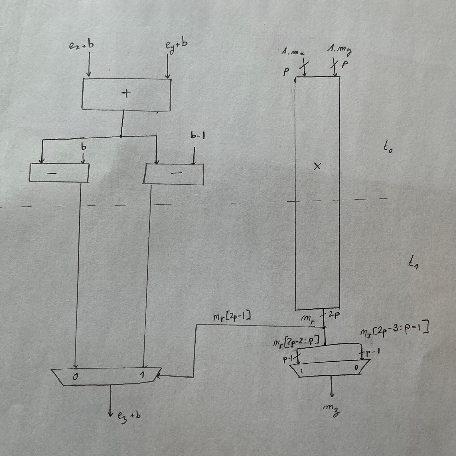
This split architecture is called the dual path architecture and has been the de facto adder architecture for high performance FPU since the 80s.
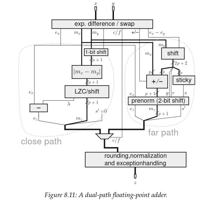
Credit: Handbook of Floating-Point Arithmetic, Second edition
Now, this schematic is actually for the IEEE compliant float, and we are not designing the general case. So how does this change for us ?
Recall how we were doing RZ rounding only ? RZ is an effective clamping of the mantissa whenever rounding is involved, which means we will never need to round upwards, which in turns means we can chop off all the logic to this effect.
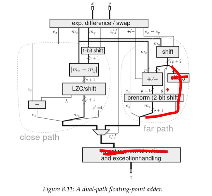
Next, since we are imposing no NaNs or \(\infty\) be used as an operand, we have no way of triggering an exception, so this too is removed.
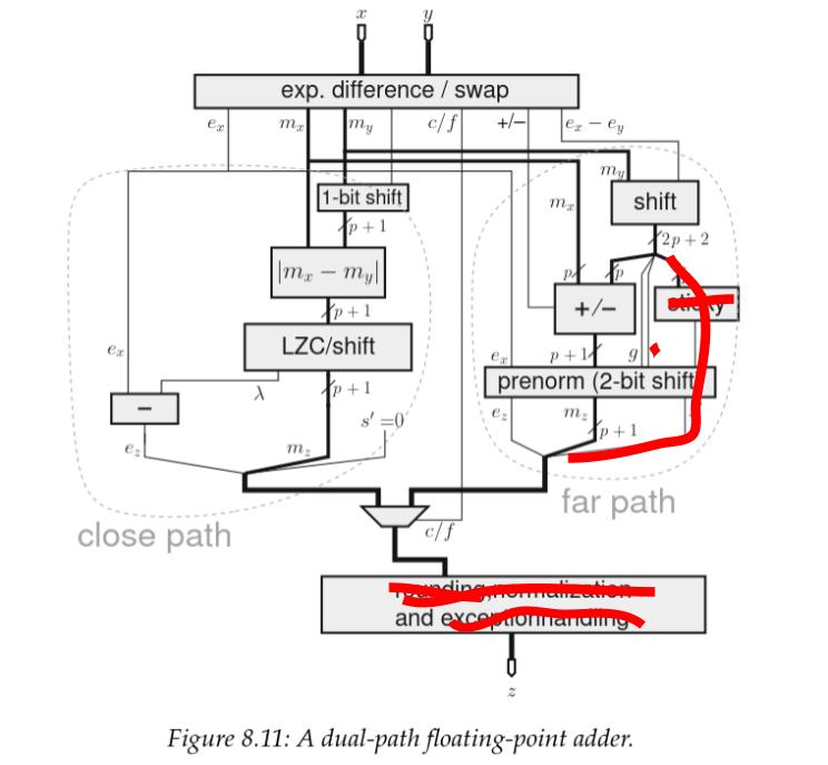
Now, this schematic doesn’t illustrate how subnormals are handled, but our implementation is also saving logic there. That said, we do still need some logic to detect when they occur and clamp them to \(0\). On the close path this functionality is rolled into a block that I will label as “normalize” that is on our critical path after the multibit significant shift and the exponent subtraction.
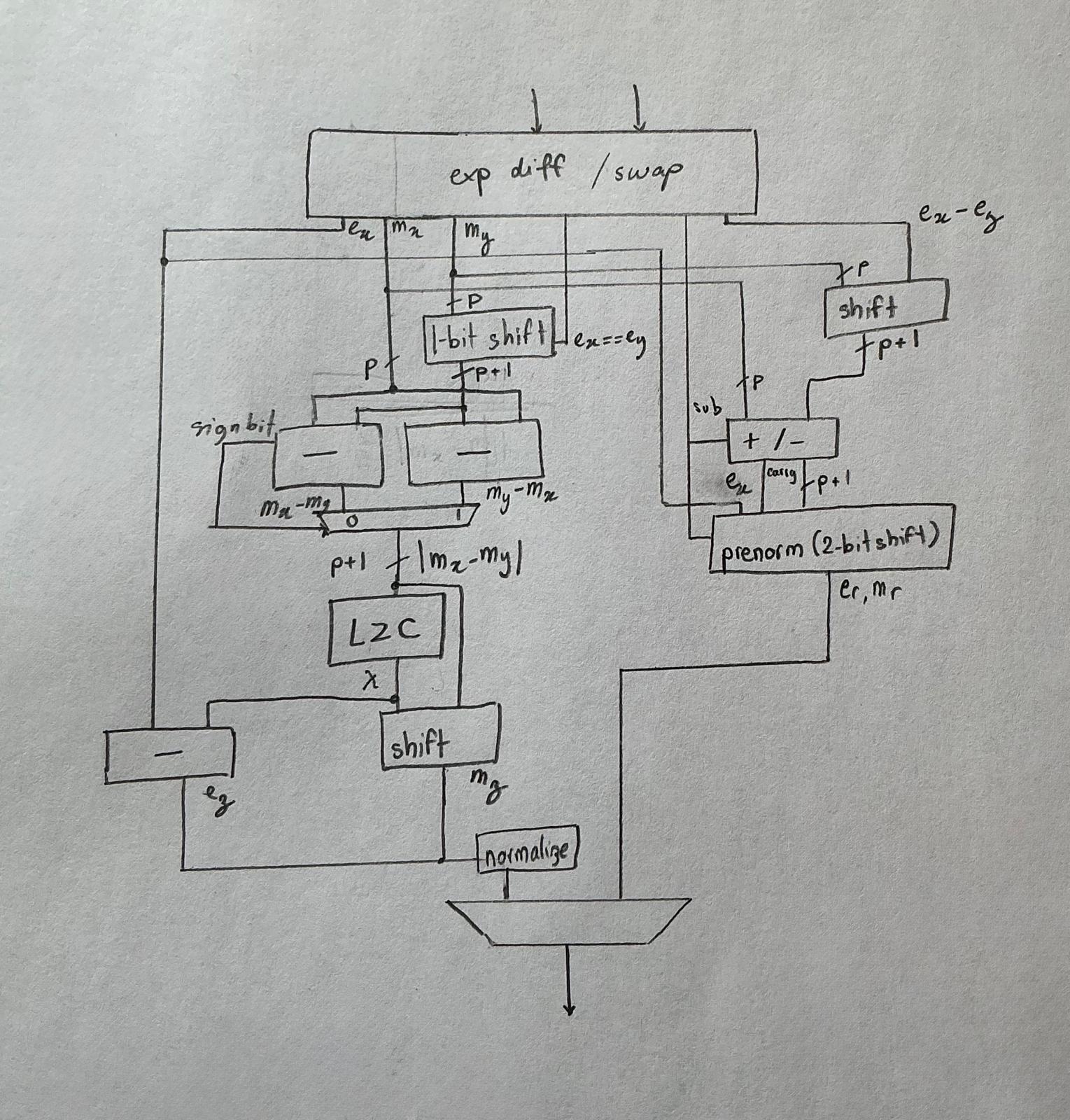
The final design looks something like this:
Chapter 3: Theory meets reality#
Verification#
Theory is entertaining but unless it has proven it can stand up to reality, nothing proves it true. So, there is no better way of validating one’s understanding than tossing it against hard cold reality.
Also, this isn’t just some thought experiment, we are actually taping this out on actual silicon, and if my past traumas with hardware have ingrained but one lesson in my mind it is that: until you have proven it works, it is broken!
Time to run some tests!
Testing floating point arithmetic hardware is actually an interesting challenge since it is full of corner cases: you can’t just test 100 random values and call it a day. No, you need exhaustive coverage for all these corners, most of which you didn’t know existed. This is very much a “you don’t know you don’t know” problem. So, what is the plan for this ?
This is where I committed my crime against verification: directed simulation driven testing scales with the size of the input space, which is a fancy way of saying it doesn’t scale linearly. This is why formal methods are increasingly widespread for floating point validation. If we wanted to test this using directed testing we would need to test for all \(2^{32}\) input combinations, which sounds like a terrible idea …
… and exactly what I am going to do because it is the only way to exhaustively test all the corner cases without having verified prior knowledge of where all the angles are.
This is a second order of ignorance problem.
This creates our next problem: testing time, just how long is testing +4 billion combinations going to take? Because I believe low iteration times is paramount to getting shit done I need this testbench to run fast, so I need a fast simulator and golden model.
Enter verilator, similarly to Synopsis vcs it compiles your simulation into an executable that can be run natively on your machine, making it the fastest open source simulator in town.
Next comes the golden model, and it just so happens we are living in 2026 and the C++23 standard library has introduced the bfloat16 type in stdfloat.
Finally, we can use the DPI-C interface (and not the slower VPI interface) to call our custom golden models coded in C++ and compiled into the testbench.
Sounds like a perfect plan … until C++ betrayed me.
How does stdfloat’s bfloat16 actually work ?#
But before going into how my golden model turned out to be not so golden, we need to understand how the stdfloat bfloat16 type actually works under the hood.
Crucially my computer actually doesn’t have native bfloat16 hardware, so how is it mathing ?
Lets test it using a simple addition:
#include <stdfloat>

int main(){
	bfloat16_t a,b,c;
	a = 1.0;
	b = 1.0;
	c = a + b;
	return 0;
}
Looking at the disassembly of this test program we can see that gcc handles the bfloat16 addition by using the soft bfloat16 floating point function replacements (__extendbfsf2, __truncsfbf2 + wrapper code ).
This is indicative that my current hardware either doesn’t have hardware support for bfloat16 or that the support isn’t being advertised to the compiler.
4	int main(){
   0x0000000000001119 <+0>:	push   %rbp
   0x000000000000111a <+1>:	mov    %rsp,%rbp
   0x000000000000111d <+4>:	sub    $0x20,%rsp

5		bfloat16_t a, b, c;
6
7		a = 1.0;
   0x0000000000001121 <+8>:	    movzwl 0xee4(%rip),%eax        # 0x200c
   0x0000000000001128 <+15>:	mov    %ax,-0x6(%rbp)

8		b = 1.0;
   0x000000000000112c <+19>:	movzwl 0xed9(%rip),%eax        # 0x200c
   0x0000000000001133 <+26>:	mov    %ax,-0x4(%rbp)

9		c = a+b;
   0x0000000000001137 <+30>:	pinsrw $0x0,-0x6(%rbp),%xmm0
   0x000000000000113d <+36>:	call   0x1180 <__extendbfsf2>
   0x0000000000001142 <+41>:	movss  %xmm0,-0x14(%rbp)
   0x0000000000001147 <+46>:	pinsrw $0x0,-0x4(%rbp),%xmm0
   0x000000000000114d <+52>:	call   0x1180 <__extendbfsf2>
   0x0000000000001152 <+57>:	movaps %xmm0,%xmm1
   0x0000000000001155 <+60>:	addss  -0x14(%rbp),%xmm1
   0x000000000000115a <+65>:	movd   %xmm1,%eax
   0x000000000000115e <+69>:	movd   %eax,%xmm0
   0x0000000000001162 <+73>:	call   0x1250 <__truncsfbf2>
   0x0000000000001167 <+78>:	movd   %xmm0,%eax
   0x000000000000116b <+82>:	mov    %ax,-0x2(%rbp)

10
11		return 0;
   0x000000000000116f <+86>:	mov    $0x0,%eax

12	}
   0x0000000000001174 <+91>:	leave
   0x0000000000001175 <+92>:	ret
Based on this assembly, the expected behavior for the bfloat16_t would be
similar to a clamped down float32_t.
Which is totally legal, given the bfloat16 behavior is not fully outlined by any spec, making it implementation defined. 🌈
Probing the standard library soft bfloat16_t’s implementation#
Since I am not perfectly fluent in x86 assembly, I decided to write a simple test program to probe out the behavior of my soft bfloat16_t.
From this I learned that it:
- has subnormal support
- has
NaNsupport - has inf support
So naive me thought that, in order to use this as a golden model for the hardware, all I needed was to also manually clamp subnormals to 0 and not drive NaNs and \(\infty\)s.
#define IS_SUBNORMAL(x) ((isnormal(x) | isnan(x) | isinf(x) | (x == 0e0bf16))) Betrayed by C++#
So I clamped my subnormals and went on my merry way.
But while I was blissfully working my way through testing all of my possible operands combinations, disaster struck.
I quote from the C++ 2022 published proposal on “Extended floating-point types and standard names” :
7.2. Supported formats
We propose aliases for the following layouts:
- [IEEE-754-2008] binary16 - IEEE 16-bit.
- [IEEE-754-2008] binary32 - IEEE 32-bit.
- [IEEE-754-2008] binary64 - IEEE 64-bit.
- [IEEE-754-2008] binary128 - IEEE 128-bit.
- bfloat16, which is binary32 with 16 bits of precision truncated; see [bfloat16]. <–
Let’s make a deal and collectively pretend we all agree we didn’t see that the spec is saying binary32 has 16 bits of precision instead of 24. This is just a typo, and I am unworthy of telling the guys literally designing the next C++ standard that they should fix their spec.
Essentially, this means bfloat16_t is, exactly like our reading of the binary hinted at: a truncated down float32_t (referred to as binary32 in the IEEE spec).
The problem with this approach is that, float32_t has a much larger internal precision \(p\) when compared with bfloat16_t :
float32_t\(p = 24\)bfloat16_t\(p = 8\)
In practice, this means that, if I want my hardware to correctly match the golden model, as specified by the C++ standard library, I will need to support \(p = 24\), which directly translates to a much wider significant path everywhere … and that is in no universe the outcome I am interested in.
Within 1 ulp#
Given the C++ standard’s library’s implementation of bfloat16_t of using a float32_t under the hood I cannot cleanly match the results of my golden model to the expected RTL output.
This is because float32_t has \(p=24\) bits on internal precision, while bloat16_t has 8 bits, so given the same input values, if the difference in exponent between these inputs if within range \(]p_{bfloat16}; p_{float32}[\)!
I will observe a difference in rounding behavior even if we are using the same rounding mode and the same operands.
Another property of this is that, this difference will be contained within a margin of the next consecutive floating point number.
To help simplify the following section, let me define \(ulp(x)\) as the “unit of last place”, or more formally :
\(ulp(x)\) is the gap between the two floating-point numbers nearest to \(x\), even if \(x\) is one of them.
As such, my relative error between my golden model’s bfloat16_t and my implementation will be at most \(1 \times ulp(x)\).
\(ulp(x)\) is defined as :
For my bfloat16 implementation with \(p=8\) we thus have \(ulp(x) = 2^{-7}\), and I will be calculating the relative error as:
C++ isn’t at fault#
Now that I have finished ranting and gotten my golden model to behave, I would like to point out that I recognize that emulating bfloat16 from float32 is the superior approach for the standard library. It allows offloading most of the compute to the CPU’s FPU, giving orders of magnitude better performance than if it was entirely implemented in software.
Sure it might come with different results, but this is what we signed up for when we started using bfloat16.
Implementation#
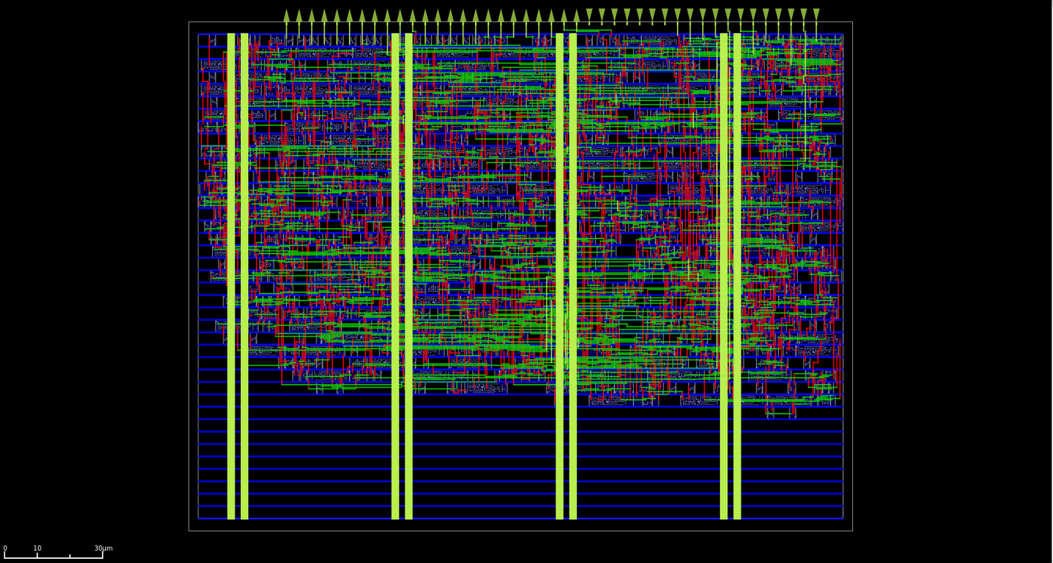
Now that we have some working bfloat16 arithmetics comes my favourite part: building it out of expensive crystals semiconductors
Captured using OpenROAD global placement in debug mode.
Since this article is focused on the floating point arithmetic I will contain my desire to tell you all about the rest of the accelerator and lock it up in the ASIC’s repo:
This design features two clock trees, one for the MAC and another for the JTAG TAP. The MAC clock targets a 100 MHz maximum operating frequency, but current output GPIO frequency experiements suggest a 75 MHz maximum, and the JTAG 2 MHz.
Tiny Tapeout ihp26a#
This time we will be taping the chip on IHP’s fancy 130nm sg13g2 node using Tiny Tapeout’s ihp26a chip as our shuttle. Also, for full transparency I was offered a coupon by the Tiny Tapout team that I traded for the area that I am using in this project (and a devboard ). So technically speaking this tapeout is sponsored by Tiny Tapeout, which will definitely not help me rave less about them!
Thanks guys!
ihp26a render.Source: https://github.com/TinyTapeout/tinytapeout-chip-renders
The IHP 130nm cell library we are using this time is special: it is lightning fast compared to the other two open source PDKs allowing us to reach some truly impressive fmax’s. (As illustrated by our fmax competition using the sister IHP sg13cmos5l node.)
But once again, we have an IO problem: the maximum GPIO stable operating frequency is expected to be around 100MHz on input and 75MHz on the output path, meaning this systolic array is effectively bottlenecked at 75MHz. But, since the sg13g2 PDK is so fast, and closing timing at 75MHz was not challenging enough, I decided to challenge myself to target a normal frequency of 100MHz. Oh and I would also do the entire bfloat16 addition and multiplication in a single cycle.
Sure, I could pipeline these operations, but that would be wasting an opportunity to force myself to improve the implementation’s performance.
Yosys you pleb#
Let me tell you about an interesting story that occurred during implementation.
But before let us set the stage: the critical path cuts exactly where you would expect it: going through the multiplication’s mantissa multiplication and continuing through the adder’s close path right through the LZC (leading zero count).
At this point in our story, I had already pulled a handful of the more classic RTL timing optimization tricks and was sitting comfortably at +0.6ns of slack on the slow corner and +3.9ns on the nominal corner. I thought my work here was done when a friend started questioning me about my LZC design choice.
I had chosen to implement a tree based LZC, the same one you find in the literature, and although the verilog code is so unreadable RTL code it warrants it’s own testbench its underlying concept was too elegant to pass up.
And so my friend comes along and suggests we do something different. Forget the tree based LZC, just write a priority mux and let the synthesizer deal with it.
always @(*) begin
        casez (in)
            9'b1????????: shift_amt = 4'd0;
            9'b01???????: shift_amt = 4'd1;
            9'b001??????: shift_amt = 4'd2;
            9'b0001?????: shift_amt = 4'd3;
            9'b00001????: shift_amt = 4'd4;
            9'b000001???: shift_amt = 4'd5;
            9'b0000001??: shift_amt = 4'd6;
            9'b00000001?: shift_amt = 4'd7;
            9'b000000001: shift_amt = 4'd8;
            default:      shift_amt = 4'd0;
        endcase
    end
In all transparency, I did NOT think this would result in better timing than the tree based LZC. Yet, between the RTL and timing there is yosys with its 124 levels of optimization, and yosys is techmap aware.
For reference, this is the original module’s code, isolated into its own module so that I can keep track of it when keeping the hierarchy during implementation :
module pmux(
        input wire [8:0] data_i,
        output reg [3:0] zero_cnt
);

always @(*) begin
        casez (data_i)
            9'b1????????: zero_cnt = 4'd0;
            9'b01???????: zero_cnt = 4'd1;
            9'b001??????: zero_cnt = 4'd2;
            9'b0001?????: zero_cnt = 4'd3;
            9'b00001????: zero_cnt = 4'd4;
            9'b000001???: zero_cnt = 4'd5;
            9'b0000001??: zero_cnt = 4'd6;
            9'b00000001?: zero_cnt = 4'd7;
            9'b000000001: zero_cnt = 4'd8;
            default:      zero_cnt = 4'd0;
        endcase
end
endmodule
This module is implemented to a 19 cell result that comes out to only 3 logic levels deep on the critical path, resulting in better timing.
In the final flattened version this results in a +0.05 ns improvement on the slow path. On one hand, this isn’t a huge gain. But on another, this experience forces me to recognise how performant the tools can be.
This casez LZC design is not only slightly faster, its biggest strength is in how much simpler it is to understand, which in turn will make it easier to maintain, directly reducing the likelihood of bugs being introduced in the future.
Sometimes a good design is about more than just performance.
Combo!#
But wait! There was a second tapeout ?!
When I started planning this article, my hope was to have the bfloat16 arithmetic be taped out as part of my second generation systolic array on IHP 130 nm.
But in the midst of writing this article the Tiny Tapeout community got the chance to do a second tapeout on IHP 130 nm targeting IHP’s newer sg13cmos5l node.
Just like how we got the chance to do the GF180 tapeout for the first generation systolic array this was a private experimental shuttle, making us come full circle.
ihp0p4 chip render.Credit: Luis Eduardo Ledoux Pardo
Now I have a somewhat unique rule for my tapeouts: I never tapeout the same design twice.
So if I wanted to submit to the ihp0p4 shuttle chip, I couldn’t just re-use my existing IP. No, I needed something new.
Enter the fmax challenge!
Do you recall how I told you IHP cells were lightning fast and how I was doing the full addition and multiplication in a single cycle ? Well part of me was dying to know how high I could reach if we were to ignore the IO limitation and aim for the maximum frequency!
Luckily for me another community member was taping out a comparable design: and so we raced!
In order to increase the frequency the bfloat16 multiplication was cut into 2 cycles. As expected, the main critical path went through the mantissa multiplication. Now, in the original implementation of the multiplication, I was using the synthesizer implementation directive to infer an unsigned Booth radix-4 multiplier.
As the LZC experience has shown us, yosys is not a light weight when it comes to generating optimized logic. Unfortunately, we trade this for a loss of control on our netlist, and in this case the inability to choose exactly where we would split the multiplication.
Thus, in order to help pipeline this path, I needed to re-implement a custom 8-bit unsigned Booth radix-4 multiplier from scratch.
Oh, also, I forgot to mention one small thing: this shuttle was officially announced, opened and closed within the span of 24 hours! So now picture all of this happening at 3am. 🫠
Inside this custom multiplication stage, a flop is added after the encoding stage, in the middle of the compression stage. We are storing the partial compression of the first two partial products, and the last 3 before, on the next cycle compressing them together to get the final result of this mantissa multiplication.
A few additional such optimizations were performed throughout the multiplier allowing this design to reach a maximum operating frequency of 454.545 MHz.
Closing#
After over half a decade, I have finally slayed my dragon and taken my revenge on floating point math!
After having build my own floating point arithmetic from scratch I now believed the only people that truly understand floating point are :
- The people writing the IEEE 754 spec
- The math PhDs working on the floating point representation
After having re-implemented floating point arithmetics and taped it out twice, I can confidently assert that I do not deeply understand floating point arithmetics, but at least now I know exactly how deep the rabbit hole goes and what I must do if I want to truly master it.
But with two 130nm tapeouts containing my own floating point IP I can confidently leave the explorations of the other minifloats and implementation of more complex operations to some other day.
Because I now have something much more important to do!
Before we can go to sleep, before we can finish writing the doc, there is one post tapeout tradition that must never be skipped:

P.S#
I highly recommend the excellent book “Handbook of Floating-Point Arithmetic, Second edition”, for readers looking for the 600 page version of the floating point question.
Special thanks to my best half, yg, Prawnzz and Erstfeld for helping review this article.